Introduction to Pharmaceutical Analysis

Free pharmacy material

Introduction to Pharmaceutical Analysis

INTRODUCTION

The pharmaceutical analysis is a branch of chemistry, which involves the series of process for the identification, determination, quantitation, and purification. This is mainly used for the separation of the components from the mixture and for the determination of the structure of the compounds. The different pharmaceutical agents are as follows:

Plants
Microorganisms
Minerals
Synthetic compounds

Based upon the determination type, there are mainly two types of analytical methods. They are as follows:

Qualitative analysis: This method is used for the identification of the chemical compounds.
Quantitative analysis: This method is used for the determination of the amount of the sample.

Types of Analytical Methods

Analytical methods are mainly of the following two types:

Classical methods:

Gravimetry—the weight of the sample is determined after the precipitation.
Titrimetry—the volume of the solution is determined after the reaction such as neutralization, complex formation, precipitate formation, and oxidation and reduction.
Volumetry—the volume of the gas evolved by the reaction is determined.

Instrumental methods:

Electrochemical methods—used for the measurement of the current, voltage, or resistance.

Examples:	Conductometry—measurement of the conductance
	Potentiometry—measurement of the potential
	Coulometry—measurement of the current
	Voltametry—measurement of the current at specified voltage

Optical methods—based upon the measurement of radiation absorbed or emitted

Examples:	Absorption methods—visible, Ultraviolet (UV), Infrared (IR), Atomic Absorption Spectroscopy (AAS)
	Emission methods—plasma emission spectroscopy, flame spectroscopy, and fluorimetry

Chromatography—paper, High Pressure Liquid Chromatography (HPLC), Gas Chromatography (GC), ion exchange, Thin Layer Chromatography (TLC), and column chromatography

Thermal methods—Differential Thermal Analysis (DTA), Thermogravimetric (TG), and Differential Scanning Calorimetry (DSC)

Other methods—X-ray diffractometry, radioactive methods, mass spectrometry, refractometry and polarimetry.

Factors Affecting the Analytical Methods Selection

Type of the analysis whether it is elemental or molecular or atomic or the other.
Nature of the material.
The precision and accuracy required for the analysis of the sample.
The time available for the analysis of the sample.
The concentration range of the sample.
Availability of the standard for the sample.
The facilities available for the analysis of the sample.

INTRODUCTION TO TITRIMETRY

Titrimetry is the volumetric procedure for the determination of concentration of the sample by the addition of the known concentration or volume of the standard substance. This reacts quantitatively with the sample solution. Then a chemical substance is used to detect the end point by the colour change or by the precipitate or complex formation at the equivalent point of the titration. This substance is known as the indicator.

The following are the general terms used in the titrimetry:

Titrant: This is a solution of the known concentration of the standard substance, which is added to the sample solution from the burette.
Titrand: This is a solution of the unknown sample whose concentration is to be determined.
Equivalence point: This is a point where the reaction between the titrant and titrand are completed and it can be detected by the colour change of the indicator.

Types of Titrations

The types of titrations can be classified based on the following:

Based on the measurement:

Volumetry: This is nothing but the measurement of the volume of the titrant required to complete the reaction.
Gravimetry: This is nothing but the measurement of the weight of the titrant required to complete the reaction.

Based on the nature of the titrant used:

Aqueous titrations: These titrations are based upon the titration of the sample solution by using the aqueous titrants such as hydrochloric acid and sodium hydroxide.
Non-aqueous titrations: These titrations are based upon the titration of the sample by using the non-aqueous titrants such as dimethyl formamide.

Based on the principle of titration:

Acid-base titrations: These titrations are based upon the titrations of the acidic or basic compounds by the consequent acids or bases.

Examples:	Titration of HCl with the NaOH
	Titration of the KOH with the HCl

These reactions are mainly based upon the reactions of the hydrogen ion and hydroxide ion to form water.

H++OH−

H2O

Example: NaOH + HCl

NaCl + H2O

Here, any free base or acid is neutralized by its subsequent acid or base.

Based on the acid or base to be neutralized, again these reactions are classified into the following two sub classes:

Acidimetry: Titration of free bases or salts of weak acids with a strong acid.
Example: Titration of strong base (NaOH) with acid (HCl)
Alkalimetry: Titration of free acids or salts of weak bases with a strong base.
Example: Titration of weak acid (acetic acid) with strong base (NaOH).

Applications of acidimetry and alkalimetry are as follows:

Alkalinity determination in water.
Determination of acid content in wine or fruit juice.
Determination of acid content in milk.
Determination of Total Acid Number (TAN) and Total Base Number (TBN) in petroleum products, edible or inedible oils and fats.
Determination of boric acid in cooling fluids of nuclear power stations.
Determination of free or total acidity in plating baths.
Determination of active ingredients in drugs or raw materials for the pharmaceutical industry.
Total nitrogen determination using the Kjeldahl technique.

Oxidation-reduction titrations: These reactions are mainly based upon the oxidation-reduction reactions by using oxidizing or reducing agents.

Example:

Permanganate titrations—these reactions are commonly known as redox reactions. By name itself it indicates the change of the oxidation state or transfer of electrons of the reactants by the use of oxidizing or reducing agents.

Oxidizing agents: Iodine, potassium dichromate, potassium permanganate solutions, Cerium IV salts, hydrogen peroxide, oxidized chlorine, for example, ClO- , ClO2.
Reducing agents: Sodium thiosulphate solutions, oxalic acid, ammonium iron (II) sulphate (Mohr's salt), hydrogen peroxide, phenylarsine oxide (PAO).

Applications of redox titrations are as follows:

Determination of Chemical Oxygen Demand (COD) of water.
Determination of oxidation capacity of water by permanganate.
Determination of free and total SO2 in water, wine, alcohol, dried fruit, etc.
Vitamin C determination.
Titration of copper or tin using iodine.
Titration of chromium VI.
Determination of water in hydrocarbons.

Complexometric titrations: These titrations are mainly based upon the complexation reactions by using the complexing agent such as the titrant.

Example:

EDTA titrations—these reactions are carried out by complex formation by combining ions by using complexating agents like Ethylenediaminetetraacetic Acid commonly known as EDTA. The end point is detected by using metal ion detectors.

2CN− + Ag+

{Ag(CN)2−}

Applications of complexometric titrations are as follows:

Total hardness of water (Ca2+ and Mg2+).
Determination of Cu2+, Ni2+, Pb2+, and Zn2+ in plating baths.
Determination of Ca2+ and Mg2+.

Precipitation titrations: These titrations are mainly based upon the precipitate formation by using the precipitating agents.

Example: AgCl titrations—these reactions are carried out by the formation of precipitate by combining the ions by using the precipitating reagents.

Ag++Cl

AgCl−

Applications of precipitation titrations are as follows:

Determination of chloride in water.
Determination of chloride in many finished products (cooked meats, preserves, etc.).
Determination of chloride in dairy products.
Determination of silver in various alloys (for jewellery).
Titration of halides.

Non-aqueous titrations: These titrations are mainly based upon the titrations by using the non-aqueous titrants.

Example: Titrations using perchloric acid and sodium methoxide.

Conditions Required for the Titrimetric Analysis

The reaction should be simple, which can be easily expressed by a simple chemical equation.
Example: Titration of NaOH with HCl which can be expressed by a simple equation.
NaOH + HCl NaCl + H2O
The titration should be relatively fast.
The end point should be detected by physical or chemical change.

Examples:	Colour change
	Precipitate formation
	Complex formation

Standard Solution

This contains the known weight of the reagent in a definite volume of the solution, which has the standard concentration. The concentration is expressed by the following terms:

Formality (F): The number moles of solute per litre of solution with regardless to the chemical formula of the compound.
Molarity (M): The number of moles of solute per litre of solution with regard to chemical formula of the compound.
Molality (m): The number of moles of the solute in 1 Kg of the solution.
Normality (N): The number of equivalents of the solute in 1 litre of the solution.
Equivalent weight (EW): The weight of the one equivalent compound.

The following standard solutions are used in the titrations:

Primary standard: This is the pure form of the substance with equivalent weight.

Examples:	Potassium hydrogen phthalate
	Succinic acid
	Sodium carbonate
	EDTA

The primary standard should have the following requirements:

It should be stable.
It should be completely soluble in the solvent.
Its purity can be determined by the standard analytical methods.
The reaction with the standard solution should be stoichiometric reactions.

Secondary standard: This is a solution, which is previously standardized by the titrating with the primary standard.

Examples:	Sodium thiosulphate
	Oxalic acid
	Copper sulphate

The secondary standard should have the following requirements:

The concentration of the secondary standard should be stable for a long period of time.
It should rapidly react with the analyte.
It should produce the sharp end point.
It should complete the reaction by the simple chemical equation.

Indicator: These are very weak organic acids or bases. Based on the hydrogen ion concentration present in the solution the indicators produce different colours. These are as follows:

One-colour indicator:
Example: Phenolphthalein which produce pink colour
Two-colour indicator:
Example: Methyl orange which produces red to yellow colour
Mixed indicator:
Example: Natural red and methylene blue

INTRODUCTION TO ELECTROANALYTICAL METHODS

The electroanalytical methods are based upon the determination of the electrical properties of the compounds. These properties include the current, potential, conductance, and voltage. At first, Michael Faraday proposed the law of electrolysis, which states that the amount of the substance deposited on the electrode is directly proportional to the weight of the substance deposited. The electroanalytical methods are of two types they are:

Interfacial methods:

Static methods:
Example: Potentiometry
Dynamic methods:

Controlled potential methods:

Examples:	Amperometry
	Voltametry

Constant current methods:

Example: Coulometry

Bulk methods:

Example: Conductometry

The principles used in the electroanalytical methods are as follows:

Potentiometry: This is mainly used in the determination of potential of sample solution when the electrodes are immersed in the solution. These are of two types:

Direct potentiometry: In this the potential is determined by using the Nernst equation, which is directly proportional to the analyte concentration.
Indirect potentiometry: This is mainly used for the determination of the change in the potential, which is noted as the end point.

Coulometry: This is mainly used for the determination of the quantity of electricity or current.
Voltametry: This is also used for the determination of the current. The only difference is by altering the potential. The change in the current flow is measured.
Conductometry: This is mainly used for the measurement of the conductance.

Laws Governing the Electroanalytical Methods

Nernst equation: The main theory involved in the potentiometry is when the known potential electrode immersed in the sample solution and then the potential is given by the Nernst equation.
E = E0 + (0.592/n) log c
where E = potential of the solution; E0 = standard electrode potential; n = valency of the ions; c = concentration of the sample solution; 0.0592 = value obtained from the RT/F.
where R = Gas constant; T = temperature in Kelvin's constant; F = faraday's constant.
Ohm's law: This law states that the current (I) is directly proportional to the electromotive force (E) and inversely proportional to the resistance (R) of the conductor.
I = E/R
The conductance (C) is defined as the reciprocal of the resistance. The resistance is expressed by the following formula:
R = ρl/A
where ρ = resistivity; l = length; A = cross section area of the homogenous material.
Therefore,
C = 1/R
= k/lA
where k = conductivity; l = length; A = cross section area of the homogenous material.
Faraday's first law:
where Q = consumed current; Mr = relative molecular weight.
Fick's second law: The total current flowing is as follows:
I =Id +Im
where I = total current; Id = diffusion current; Im = migration current.

The Fick's second law states the diffusion rate of the ion on the electrode surface is as follows:

δc/δt = Dδ2/δx2

where D = diffusion co-efficient; C = concentration; t = time; x = distance from the electrode surface.

Electrodes Used in the Electroanalytical Methods

There are mainly three types of electrodes used in the electroanalytical methods. They are as follows:

Working electrode: This is used as an indicator electrode to indicate the change in the sample concentrations.

Examples:	Hydrogen electrode
	Glass electrode

Reference electrode: This is used to produce the standard constant potential and is not affected by the sample concentration.

Examples:	Saturated calomel electrode
	Silver electrode

Auxiliary electrode: This is used as counter electrode, which is used in the three electrode system. This is mainly used in the voltametric determinations.

Example: Standard hydrogen electrode

INTRODUCTION TO SPECTROSCOPY

Spectroscopy is the branch of science, which deals with the study of interaction of the electromagnetic radiation with sample substances. The interaction is mainly based upon the absorption or emission of the radiation by the sample. The absorbed or emitted radiation is in the form of quantum energy. Generally the spectroscopy is defined as the measurement and interpretation of the electromagnetic radiation absorbed or emitted by the sample. This is used for the measurement of the radiation absorption or emission in the atomic or molecular level. The spectroscopy is divided into the following types.

Based on the atomic or molecular level:

Atomic spectroscopy: This is mainly used in the study of the electromagnetic radiation in the atomic level.

Examples:	Atomic absorption spectroscopy
	Flame photometry

Molecular spectroscopy: This is mainly used in the study of the electromagnetic radiation in the molecular level.

Examples:	UV spectroscopy
	Visible spectroscopy
	IR spectroscopy
	Fluorimetry

Based on the absorption or emission of the radiation:

Absorption spectroscopy: The absorbed radiation is measured in this spectroscopy.

Examples:	UV spectroscopy
	Visible spectroscopy
	IR spectroscopy
	Fluorimetry
	Atomic absorption spectroscopy

Emission spectroscopy: The emitted radiation is measured in this spectroscopy.

Examples:	Flame photometry
	Fluorimetry
	Atomic emission spectroscopy

Electromagnetic Radiation

The energy propagates through the substance as the electromagnetic waves such as UV rays, IR rays, X-rays, or gamma rays. This radiation shows the reflection, refraction, or diffraction.

Wavelength diagram (The distance between the two successive waves)

Electromagnetic radiation consists of photons of different energies with different spectral regions as shown in the figure.

Wavelength ranges of different spectrums

Electromagnetic waves are usually described in terms of the following:

Wavelength (λ)—distance between two successive peaks.
Wave number (υ)—number of waves per cm.
Frequency (λ)—number of waves per second.

The arithmetic relationship of these three quantities is expressed by,

c = λυ

The laws of quantum mechanics may be applied to photons to show that,

E = hυ

where E = energy of the radiation; v = frequency; h = Planck's constant.

Combining the above two equations, we get,

E = hc/λ

The radio frequencies are removed from the incident light by the absorption. This is observed by the excitation of the molecules from the ground state to the excited state.

Examples:	UV
	Visible
	IR

The radio frequencies are emitted when the excited molecules return to the ground state.

Examples:	Fluorimetry
	Chemiluminescence

The Electromagnetic Spectrum

Generally, when light falls upon a homogenous medium reduction of the intensity of the light may occur due to the following reasons:

A portion of the incident light is reflected.
A portion is absorbed within the medium.
Remaining is transmitted.

I0 =Ia +It +Ir

where I0 = intensity of incident light; Ia, It, and Ir = intensity of absorbed, transmitted, and reflected light, respectively.

Convertion of incident light

Generally, reflection is not observed in case of clear medium. The change of absorption of light with the thickness of the medium is given by Lambert and the extended concepts are developed by Bouguer. Beer later applied it to the different concentrations. The two separate laws governing absorption are known as Lambert's law and Beer's law. It is together known as Beer-Lambert's law.

Beer's Law

The intensity of a beam of monochromes in light decreases exponentially with increase in the concentration of absorbing species arithmetically. In quantitative analysis, which is mainly concerned with solutions, Beer studied the effect of concentration of the coloured constituent in solution upon the light transmission (or) absorption.

-dI/dc∞I

where I = intensity of incident light; dI = decrease in the intensity of incident light; dc = decrease in the concentration.

dI/dc = KI

where K = proportionality constant.

dI/I = Kdc

On integration, we get,

–ln I – Kc + b (b = Constant of integration) (1)

When concentration is ‘0’, there is no absorbance hence I = I0

–ln I0 = K x 0 + b

–ln I0 = b

By substituting the ‘b’ value in equation (1)

–ln I = Kc – lnI0

ln I0 – ln I = Kc

ln I0/I = Kc (∴ log x – log y = log x/y)

I 0/I = eKc

On inverse on both sides

I/I0 = e−Kc

I = I0 e−Kc Beer's law

Lambert's Law

The rate of decrease of intensity of incident light with the thickness of the medium is directly proportional to the intensity of incident light that is equivalent to the intensity of emitted light decreased exponentially as the thickness of the absorbing medium increases arithmetically.

-dI/dt∞I

where dI = decrease in the intensity of incident light; dt = decrease in the thickness of the medium.

Same as Beer's law we will get the

I = I0 e−Kt Lambert's law

By combining both Beer's and Lambert's equations, we get

I = I0e−Kct

I = I0 10 −Kct (Converting natural logarithm to base 10)

I/I0 = 10-Kct

On inversing both sides,

I0/I = 10−Kct

log I0/I = Kct (taking log on both sides)

The quantity log I0/I is called as absorbance (A) and it is equal to the reciprocal of the common logarithm of transmittance (T)

A = log 1/I/I0

Therefore

A = log I0/I

T = log I/I0 = KCt

A = KCT

Beer-Lamber's Law

When ‘C’ is in moles/Litre, the constant is called molar absorptivity (or) molar extinction co-efficient (ε)

A = ε CT

‘ε’ can also be written as,

where

is the absorbance of 1% W/V Solution using a path length of 1 cm.

Application of Beer's Law

Consider the case of two solutions of a coloured substance with concentrations C1 and C2 placed in an instrument in which the thickness of the layer can be altered and measured easily when two layers have the same colour intensity.

It1 = I010−εl1C = It2 = I010−εl2C2

where l1 and l2 = Lengths of columns of solutions.

l1c1 = l2c2

Hence, it can be possible to investigate the validity of Beer's law by varying C1 and C2 and also for the determination of an unknown concentration.

Hence, by plotting ‘A’ as ordinate against concentration as abscissa, a straight line will be obtained, which will pass through the origin. This calibration line is used to determine the unknown concentration of the solutions by measuring the absorbances.

Beer-Lambert's Law

Deviation from Beer-Lambert's Law

Generally, positive deviation (upward curve) or negative deviation (downward curve) is observed in graphs of absorbance versus concentration (Beer-Lambert's law plot) or of absorbance versus path length.

Deviation plot

Positive deviation results when a small change in concentration produces a greater change in absorbance.

Negative deviation results a large change in concentration produces a smaller change in absorbance. Several reasons for the observed deviation from Beer's law are as follows:

Instrumental deviations such as stray light, improper slit width, and fluctuation in single beam.
Effect of stray light on Beer's law plots
Chemical effects like association, dissociation polymerization, complex formation, etc., as a result of the variation of concentration.

Examples:

A solution of benzoic acid, high concentration in a simple solution has a lower pH and contains a higher proportion of unionized form than a solution of lower concentration. The ionized and unionized forms of benzoic acid have different absorption characteristics.
Hence, increasing the concentration of benzoic acid gives maximum of 273 nm with positive deviation from Beer's law and lower absorption of 268 nm with negative deviation from Beer's law.
In unbuffered solution of potassium dichromate the dissociation of the dichromate ions are observed by lowing the pH –
Methylene blue at concentration of 105 m exists as monomer and has X max of 660 nm. However, Methylene blue at concentration above 10−4 m exists as dimer which has X max of 600 nm
The Beer-Lambert's law doesn't hold when the solute forms complexes, the composition of which depends on the concentration.
In complete reactions, like insufficient time for the completion of reaction also produces deviations from Beer's law.
Example: Determination of iron uses thioglycollic acid before completion of reaction.

Instrumentation

The Plank's law states that the absorbed or the emitted radiation is directly proportional to the frequency and is inversely proportional to the wavelength. This absorbed or emitted radiation intensities are recorded by the instrument called spectrophotometer. The following are the different components of the spectrophotometers:

Radiation Source

This is mainly used for the excitation of the molecules or atoms present in the sample. They are mainly of the following two types:

Continuous sources:

Deuterium lamp
Tungsten lamp
Xenon arc lamp
Argon lamp

Line sources:

Mercury vapour lamp
Sodium vapour lamp
Hallow cathode tube
Discharge lamp

The following are the different radiation sources used for the different spectroscopic methods:

Visible spectroscopy: In this method, the main radiation sources used are as follows:

Tungsten lamp
Carbon arc lamp

UV spectroscopy: In this method, the main radiation sources used are as follows:

Hydrogen discharge lamp
Deuterium lamp
Xenon discharge lamp
Mercury arc lamp

IR spectroscopy: In this method, the main radiation sources used are as follows:

Nernst glower
Nichrome wire

Fluorimetry: In this method, the main radiation sources are as follows:

Mercury vapour lamp
Xenon arc lamp
Tungsten lamp

Nephelometry and turbidimetry: In this method, the main radiation sources use are as follows:

Tungsten lamp
Mercury arc lamp

Filters and Monochromators

The filters and monochromators are mainly used to convert the polychromatic light into monochromatic light. The polychromatic light contains the several wavelengths that are converted to single wavelength by the filters or monochromators.

Filters: These are mainly used in the visible spectroscopy. These are of the following two types:

Absorption filter: These are made up of glass coated with the pigments. This absorbs the undesired radiation and allows the desired radiation.
Interference filter: These are also known as the Fabry-Perot filters. In this type, the radiation is reflected by the film and the incident radiation undergoes the interference, which produces the monochromatic light. This is governed by the following equation:
λ = 2ηb/m
where η = dielectric constant of the material; b = layer thickness; m = order number.

Monochromators: These are more efficient than the filters. These are of the following two types:

Prism type monochromators: The prisms disperse the light radiation into monochromatic light. The resolution depends on the size and the refractive index of the prism. These are of the following two types:

Refractive type: In this type, the prism is rotated for the selection of the desired wavelength.
Reflective type: In this type, the Reflective surface reflects the radiation which converts the polychromatic radiation into monochromatic light.

Grating type monochromators: These are more efficient than the prism type monochromators which converts the polychromatic light into monochromatic light. These are mainly of the following types:

Diffraction gratings: The diffraction gratings principle is the reinforcement of the polychromatic rays which reflects the monochromatic rays. This is governed by the following equation:
mλ = b (sin i + sin r)
where m = order number; b = spacing between the grating; i and r = angle of incidence and reflection respectively.
Transmission grating: In this refraction produces the reinforcement of polychromatic light which produces the monochromatic light. This is governed by the following equation:
where d = 1/lines per cm; m = order number; θ = angle of deflection or diffraction.

The following are the different monochromators used in the different types of spectroscopes:

Visible spectroscopy: In this type filter and monochromators are used.
UV spectroscopy: In this type the grating monochromators are used.
Fluorimetry: In this type the diffraction type monochromators are used.
Nephlo-turbidimetry: In this type monochromators are used.
IR spectroscopy: In this type diffraction monochromators are used.

Sample Cells

Sample cells are generally called as the cuvettes. These are mainly made up of the glass or quartz. These are mainly used for handling the sample.

The following are the sample cells used for the different types of spectroscopic methods:

Visible spectroscopy: In this method glass sample cells are used.
UV spectroscopy: In this method quartz sample cells are used.
Fluorimetry: In this method the quartz sample cells are used.
Nephlo-turbidimetry: In this method rectangular glass cells are used.
IR spectroscopy: In this method the alkyl halide sample cells are used.
Mass spectroscopy: In this method glass test tube of 25 cm long and 5 mm outer diameter are used.

Detectors

The detectors are also called as the photometric detectors. These convert the light radiation into electrical signal which is recorded by the recorder. The most commonly employed detectors are as follows:

Photovoltaic cell detector: This is made up of silver coated thin layer, which acts as an electrode. At the bottom of this electrode one iron plate acts as another electrode. These two electrodes are separated by the selenium layer which is semiconductor in nature. When the light falls on the selenium layer, the electrons are taken by the silver layer which causes the potential difference between the two electrodes and causes the flow of current.
Photo voltaic cell
Photo tube: This consists of the glass tube containing the cathode and an anode. This is coated with the cesium, which liberates the electrons when the radiation falls on it. This movement of electrons towards the anode coated with the silver-oxide produces the current flow This has the sensitivity when compared to that of the photo voltaic cell.
Phototube
Photo multiplier tube: This is the more effective detector when compared to other detectors. The principle involved in the detector is the secondary emission of the electrons when the light falls on the cathode and the replication of the anodes. The secondary emission of the electrons produces the current signals.
Photomultiplier tube
Thermocouple: This is made by two metal wires that are welded through a joint which is maintained at different temperatures. This thermocouple is closed in an evacuated steel casing with KBr.
Bolometer: This is made by inserting the platinum strip in an evacuated glass vessel and one arm is connected to the Wheatstone bridge.
Golay cell: This is made up of gas-filled chamber which undergoes a pressure increase. This detector is more efficient than other detectors.
Pyroelectric detector: This detector works mainly based upon the principle of polarization which shows the electrical signal.

The following are the detectors used in the different spectroscopy:

Visible spectroscopy: In the above 1, 2, and 3 detectors are used.
UV spectroscopy: In this photo multiplier tube is used as the detector.
Fluorimetry: In this the photo multiplier tube is used as the detector.
Nephlo-turbidimetry: In this the photo voltaic cells, photo tubes, and photo multiplier tubes are used as detectors.
IR spectroscopy: In this the thermocouples, golay cell, bolometers, thermistors, pyroelectric detectors are used.

INTRODUCTION TO CHROMATOGRAPHY

This is the physical method, which is mainly used for the separation of the compounds when the sample is distributed between the two phases. The two phases are the mobile phase and the stationary phase. The mobile phases generally employed are the liquid and the gas whereas the stationary phase employed are the solid or liquid or gas. This method is mainly employed for the identification and separation of the compounds. These are mainly employed for the following:

To separate the mixture of compounds into individual components.
To identify the unknown samples with reference to the standard compounds.
To determine the purity and concentration of compounds.
To monitor final product formation.

Classification of Chromatography

Based on the separation mechanism: This separation is mainly based upon the nature of the stationary phase.

Adsorption chromatography: The principle is based upon the components that are adsorbed on the surface of the solid stationary phase such as silica gel.

Examples:	Thin layer chromatography
	Column chromatography

Partition chromatography: The principle is based upon the partition between the two immiscible liquids. The partition is mainly based upon the distribution co-efficient. The stationary phase is a liquid, forming a thin film on an inert solid support.

Example: Paper chromatography

These are of the following two types:

Normal phase chromatography: In this, the stationary phase is the polar and the mobile phase is the non-polar.
Reverse phase chromatography: In this, the stationary phase is the non-polar and the mobile phase is the polar.

Ion-exchange chromatography: The principle is based upon the separation of the charged particles by using the ion-exchange resins as stationary phase. These are mainly of the following two types:

Cation exchange resins:
Example: Sulfonated poly styrenes or carboxylic methacrylate
Anion exchange resins:

Example: Quaternary ammonium poly styrene or phenol formaldehyde

Size exclusion chromatography: The principle is based upon the separation of the mixture of components based on their molecular sizes. In this method, the stationary phase used is the gel and the large molecules elute first and the small molecules elute later.

Examples:	Gel permeation chromatography
	Gel filtration chromatography

Zone electrophoresis: The principle is mainly based upon the bands formation by the positively and negatively charged compounds. In this method, the stationary phase is formed as bands.

Affinity chromatography: The principle is mainly based upon the affinity of the biomolecules to the ligands. Then the ligands are separated by the suitable polysaccharides polymer like cellulose.

Chiral chromatography: The principle is mainly based upon the separation of the enantiomers by using the chiral stationary phase.

Based on the mobile phase used: This is mainly based upon the state of the mobile phase used in the separation.

Liquid chromatography (LC): In this, liquids such as aqueous solvents or organic solvents are used as the mobile phase. This is of the following two types:

Liquid-solid chromatography—where the stationary phase is the solid.
Liquid-liquid chromatography—where the stationary phase is the liquid

Gas chromatography (GC): In this, inert gases such as hydrogen or helium or nitrogen are used as mobile phase. These are of the following two types:

Gas-solid chromatography
Gas-liquid chromatography

Based on the stationary phase holding technique:

Planar chromatography: In this method the stationary phase is formed as layer. They are of the following two types:

Thin layer chromatography—where the stationary phase such as silica gel which is prepared as slurry on glass or aluminium sheets.
Paper chromatography—where the stationary phase such as fibres in the paper form is used. The commonly employed paper is Whattman filter paper.

Columnar chromatography: In this method, the stationary phase is filled or packed in the tube made up of glass or metal.

Examples:	Column chromatography
	HPLC
	GC

Based on the purpose:

Analytical chromatography: This is mainly used to determine the chemical composition of a sample. These are of the following two types:

Qualitative chromatography: This is mainly used for the determination of the quality of the product.
Quantitative chromatography: This is mainly used for the determination of the quantity of the product.

Preparative chromatography: This is mainly used to purify and collect the one or more components of sample.

Mobile Phases Used in the Chromatography

This is mainly used as solvent, developer, and as eluent. The commonly employed mobile phases in the chromatography are as follows:

Petroleum ether
Carbon tetra chloride
Cyclohexane
Ether
Acetone
Benzene
Toluene
Esters
Chloroform
Methanol
Ethanol
Water

The selection of the mobile phase is based on the following factors:

Nature of the sample
Nature of the stationary phase
Mode of the chromatography
Nature of the separation

Stationary Phase

The stationary phase is mainly used to separate the mixture of the components into individual components. The stationary phase should have the following requirements:

Should have uniform particle size and shape
Should have high stability
Should be inert
Should be inexpensive

The commonly employed stationary phases in the chromatography are silica gel, alumina, cellulose, kieselguhr-polyamide, Polydimethylsiloxane (PDMS), etc.

Detection of the Components

Detection of the components are done by the following methods:

UV-visible detector
Fluorescence detector
Flame ionization detector
Refractive index detector
By using the visualizing agents—this can be done by using the spray reagents which are specific for the compounds.

Examples:	Ferric chloride for the phenolic compounds
	Ninhydrin reagent for the amino acids
	Dragendroff's reagent for the alkaloids

STATISTICAL ANALYSIS

Introduction

The statistical analysis helps the analyst to analyse that the results obtained are as close to the theoretical values. The analyst must give the assurance that the method has the appropriate accuracy and the precision with minimization of the errors. The general classifications of the errors are as follows:

Systematic errors: These errors are also known as the determinate errors. These errors must be avoided or that magnitude must be determined. The most important types of the systematic errors are as follows:

Operational and personal errors: These are observed because of the analyst. These are mostly of the physical errors which are caused by not following the appropriate procedures.

Examples:	Mechanical loss of the material during the analysis
	Over washing of the precipitate
	Maintenance of the incorrect temperatures
	Insufficient cooling of the crucibles before weighing
	Hygroscopic materials are subjected to the moisture
	Use of the impure reagents.

The personal errors may arise from the analyst inability to make the accurate results.

Example: Some persons are unable to observe the colour changes sharply in the titrimetric analysis and more addition of the reagent.

Instrumental and reagent errors: These are observed from the use of uncalibrated instruments or the improper construction of the instruments and the use of the unpurified reagents.

Examples:	Faulty construction of the balances
	Uncalibrated weights
	Uncalibrated instruments
	Uncalibrated weights

The reactions of the reagents with the glass ware are as follows:

Reagents stability
Use of the unpurified reagents

Method errors: These are observed from the sampling errors and the incompleteness of the reaction.

Examples:	Solubility of the precipitates
	Co-precipitation
	Post-precipitation
	Decomposition
	Volatilization

The difference observed between the obtained end point and the theoretical end point.

Additive and the proportional errors: These are observed from the impurity in the standard substances and the constituents to be determined.

Example: Loss in weight of the crucible and an impurity present in the standard substance which leads to the molarity and normality changes.

Random Errors: These are observed by the same analyst when the successive measurements are made with the same identical conditions. These are also known as the indeterminate errors.

Example: Numerical errors

Minimization of Errors

The errors are minimized as follows:

Proper calibration of the glass ware, pipettes, burettes, weights, balances, instruments, etc.
The correction factors are added to the results that the calibration is not appropriate.
By running the blank with the sample. The blank solution is defined as the solution by omitting the sample addition. The blank and the sample solutions are carried simultaneously to obtain the accurate results.
By running the standard solution along with the sample unknown solution. The weight of the unknown sample solution is determined by the following equation:
The following standard substances are commonly employed:

Sodium oxalate
Potassium hydrogen phthalate
Benzoic acid
Arsenic oxide

By using the independent method of analysis.
Example: Determination of the strengths of the HCl by the acid-base titrimetry and the precipitation titrimetry.
By running the parallel determinations.
By using the standard addition method—a known amount of the constituent is added to the sample.
By the addition of the known amount of the reference material to the series of the sample material.
By using isotopic dilution method—a known amount of the radioactive isotope is mixed with the sample solution.

Significant Figures and Computation

The digits of a number that are needed to express the precision of the measurement from which the number is derived are known as the significant numbers. The digit zero is the significant figure except when it is the first digit in a number.

Example: Consider 1.0056 g, here the zero is the significant figure but in the quantity 0.025 kg the zero is not a significant number.

The rules for the computation are as follows:

The average of the significant figures of the data should give as one certain figure.
Example: The volumes of the titrant are observed between the 20.4 ml and 20.6 ml which can be written as 20.5 ml.
For the rounding of the quantities to the correct number of significant figures.
Example: The averages of the different values are given as the one such as 0.234, 0.235 and 0.236. The average is given as the 0.235.
In addition or subtraction should be in each number the significant numbers should be less.

Examples:

165.11 + 6.095 + 0.5869 then the significant numbers for this are 165.1 + 6.09 + 0.59

In multiplication or division should be in each number the significant numbers should be less.

Example: 1.26 × 0.6834 × 24.8652 then the significant numbers are written as 1.26 × 0.683 × 24.87

Accuracy

Accuracy is defined as the closeness of the practical value to that of the theoretical values or the standard values. The determination of the accuracy requires the calibration of the method with the standard substance. There are two different methods for the determination of the accuracy. They are as follows:

Absolute method: This method is carried by the varying amounts of the sample and proceeding with the specified standard instructions. Then the difference between the mean of number of results and the amount of the constituent present in the sample. This can be expressed as the parts per thousand. This method is mainly used to determine the accuracy of the method in the absence of the foreign substances.
Comparative method: This method involves the use of the secondary standard materials. This method is mainly used to measure the accuracy by at least two standard methods applied for the analysis of the sample.

Precision

Precision is defined as the repeatability or reproducibility of the results. There is distinction between the repeatability and the reproducibility.

Example: A sample is containing the 49.10 percent of a constituent A then the results obtained by two analysts by using the same substance and the same analytical method are as follows:

The analyst I results are précised because of the reproducibility of the results.
The analyst II results are not reproducible and are not précised values.

Precision determination

Absolute error:

E = xi – xt

where xi and xt are the obtained and theoretical values, respectively.

Relative error:

E = {[xi – xt]/xt} × 100

Accuracy determination

Standard Deviation

This is also called as the root mean square deviation this can be derived from the following:

The arithmetic mean is as follows:

where x1, x2, x3, and xn are the different values obtained in the method n = number of variables obtained in the method.

The standard deviation is as follows:

The square of the standard deviation is known as the variance. Then the relative standard deviation is given by,

Then the co-efficient of variation is given by,

Comparison of the Results

There are two methods for the comparing the results. They are as follows:

Student's t-test: This is a statistical hypothesis test in which the test static follows the student's t distribution. This is introduced by the William Sealy Gosset in 1908. This test is used for the small samples. This is to compare the mean from a sample with standard value and to express the level of the confidence. It is also used to test the difference between the means of two sets of data , and .
where μ = true value; n = number of variables; SD = standard deviation.
The t-test is applied for the following assumptions:

Samples are obtained randomly
The samples standard deviation is not known

The applications of t-test are as follows:

To test the significance of a single mean.
To test the significance of the two different means.
To test the significance of the observed correlation co-efficient.

F-test: This is mainly used to compare the precision of the two sets of the data that is between the two different analytical methods.
F = S12/S22

Correlation Co-efficient

This is used to correlate the linear relationship between the two variables x1 and y1. The correlation co-efficient is denoted by the r.

The correlation co-efficient value must lie between the +1 and −1.

There three main types of correlation are as follows:

Positive correlation:
Positive correlation
Negative correlation:
Negative correlation
No correlation:
No correlation

Sensitivity

It is a measure of the instrument ability to discriminate between small differences in analyte concentration. The slope of the calibration curve at the concentration of interest is known as the calibration sensitivity.

S = mc + Sbl

where m = slope of the linearity line; c = analyte concentration; Sbl = blank signal;.

Analytical sensitivity (γ)

γ = m/Ss

where m = slope; Ss = standard deviation.

Detection Limit

This limit is the minimum concentration of the sample that can be detected with a specific method of known confidence level. This is commonly known as the LOD. This is determined by the signal to noise ratio.

LOD = S/N

Quantitation Limit

The minimum concentration at which the quantitative measurements are made is known as the quantitation limit. This is the range over which the detector responds to the change in the sample concentration.

Loss on quantitation

Selectivity

This is the selectivity of the analytical method which refers to the degree of interference that is totally free.

Calibration of the Instrumental Methods

There are three methods for the calibration of the instruments. They are as follows:

Calibration curve method: The standard substance with different concentrations are measured and recorded. Then the plot is constructed between the instrumental signals versus the analyte concentration. This is also called as the line of best ft method.
Calibration curve
Standard addition method: The standard substances are directly added to the sample and measure the sample solutions. Then the results are plotted by taking the absorbance values versus volume of the sample.
Standard addition curve
Internal standard method: The internal standard substance is added to the sample solutions. Then all the samples are measured and the results are recorded. The ratio of the analyte signals to the internal standard signal is plotted as a function of the analyte concentration.
Internal standard curve

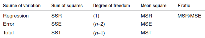
Analysis of Variance

It is the technique that the total variance present in the data is divided into the several components. These are mainly associated with the specific source of the variation. This is a parametric test. These are less complex and are very simple. These are mainly helpful in the analysis of the clinical trials. The steps involved in the ANOVA are as follows:

Calculate the sum of squares for the data.
Calculate the treatment sum of squares.
Draw the ANOVA table.

There are mainly two types of ANOVA:

One-way ANOVA: In this the following procedures are followed:

Choose the experimental design and state the null hypothesis
Define the significance level
Choose samples and perform the experiment
Calculate the total sum of squares
Construct the ANOVA table
Calculate the F static
Refer the F static value in the table
If the calculated F value is equal or greater than the two treatments are said to be differ.

Two-way ANOVA: This is mainly used more than the two samples. This is same as the one-way ANOVA.
ANOVA table

Factorial Designs

The factorial designs are used in the experiments where the effects of the different factors or conditions on the experimental results are evaluated. A factor is defined as the variables such as concentration, temperature, drug treatment, etc. The levels of factors are defined as the values assigned to the factor. Factorial designs have the following advantages:

To detect the main effects
To identify the interactions
To minimize the errors
To maintain the optimum conditions

Regression

Regression is predicting the average value of one variable which is dependent versus another variable which is independent. This is first given by Francis Galton. The simple linear regression is given by the following equation:

y = α + βx

where α = Y-intercept; β = slope of the line; y = dependent variable; x = independent variable.

Regression plot

The relationship between the X and Y is a straight line that shows the linear relationship. The relationship between the two variables is determined by the procedure known as the curve fitting. However, this is not that much efficient because of the following problems:

Must know the predicting equation.
Must know the particular equation.
Must know the merits of the analysis.

Method of Least Squares

This is used for the determination of the best ft line. In this method, the n pairs of numbers such as (x1, y1), (x2, y2) … (xn, yn) are taken. Then the equation for the line is given by,

= α + βx

Here,

is used to distinguish between the observed value (y) and the corresponding value.

y = α + βx + e

where α = Y-intercept of the population regression line; β = slope of the population regression line; e = observed errors by the residuals from the fitting the estimated regression line.

Then the sum of squared errors in regression is given by,

Then the degree of freedom in the regression is given by the formula,

df = (n – 2)

where n = total number of observations.

Then the co-efficient of the determination is the measure of the strength of the regression relationship.

Total deviation = error deviation + regression deviation

SST = SSE + SSR

R2 = SSR/SST or 1 – SSE/SST

REVIEW QUESTIONS

What are the different types of errors?
How do you minimize the errors?
Define the following:

Accuracy
Precision
LOQ
LOD

Add a note on significant figures.
How do you determine the standard deviation?
Explain about the regression.
What is the method of least squares?
What is ANOVA? Explain the table of ANOVA.
How do you calibrate the instruments?
Explain the student's t-test and the F-test.

Pharmacy Study Material